Theory

Infrastructure diagram for 2-node Quantum Key Distribution (QKD) system based on BBM92 protocol. Qcrypto (and QKDServer) fall under the ‘BBM92 software stack’.

This page houses a general overview of some pertinent QKD concepts followed by a reasonably deep dive into our code implementation of said concepts.

qcrypto in action

This section covers how key qcrypto functions are used in QKDServer. Qcrypto and QKDServer are software suites used in S-Fifteen’s implementation of the BBM92 QKD protocol for secure communication with entangled photons.

General Flow

The protocol begins with two remote parties, conventionally referred to as Alice and Bob. A photon source generates entangled photon pairs and sends half of every pair to Alice and the other half to Bob. In reality, the source may be co-located with either party, typically Alice, or be situated at its own remote location.

Upon receiving their half of the photon pair, Alice and Bob will need to record the timing of the photon arrival for later comparison with the other party. This is done by the program readevents.c.

Since each photon of a photon pair travels different paths (one to Alice and another to Bob), they experience different levels of attenuation, dispersion, polarization drift etc. Consequently, Alice and Bob will see different photon count rates despite using the same source. If the photon source is co-located with Alice, she will likely see higher count rates as the photons travel a shorter distance to reach her. Thus, Alice may be referred to as ‘high-count side’ and Bob ‘low-count side’.

After the photon arrival times are registered by readevents.c, the timestamps are sorted or chopped into appropriate time bins (hereafter epochs) by chopper.c and chopper2.c. chopper2.c operates on the high-count side and chopper.c on the low-count side. The output of chopper2.c is a single type of file that contains timing information and detector measurement results. On the other hand, chopper.c outputs two types of files. The first type is the same as chopper2.c. The second contains the basis choices in place of measurement results. The latter type is meant to be sent over to the high-count side for basis comparison purposes. File transfers between Alice and Bob is mediated over a classical channel by the transfer daemon transferd.c running on both local machines.

After chopping, pfind.c is used by both parties to find the time differences between their local clocks.

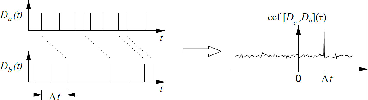
The use of a down-converted photon pair source leads to strongly correlated arrival times on both sides. Examining the cross correlation function (ccf) quickly reveals the time difference between Alice and Bob. The two graphs on the left show the arrival times of photons separately on Alice’s and Bob’s detectors.

To properly perform the BBM92 protocol, Alice and Bob must correctly identify which photons originated from the same pair. One way to do this is to have a dedicated communication channel for synchronization between both sides. However, the use of a down-converted photon source provides another option, which we implement in pfind.c.

This option takes advantage of the fact that a photon pair source that emits photons with a bandwidth of a few nanometers will have a coherence time of a few 100 femtoseconds. Then, by taking the time difference between each of Alice’s timestamps with each of Bob’s timestamps, the modal time difference will greatly exceed any other in modality. This modal time difference is the additional time that a photon from the same pair will take to reach Bob after its counterpart has already reached Alice, and it is also the value that will be passed to the next program costream.c to synchronize communications between Alice and Bob.

Mathematically, we can find this modal time difference with the cross correlation function (ccf). The ccf is similar to, but distinct from the convolution. The convolution of two functions is defined by the following equation:

\[(f \circledast g)(\tau) := \int f(t)g(\tau - t) dt\]

whereas the ccf is defined:

\[ccf[f,g](\tau) := \int \bar{f(t)}g(\tau + t) dt\]

The ccf can be thought of as a measure of overlap between two functions as one is being dragged across the other. In the equation above, the function \(g\) is dragged over \(f\) as \(t\) changes. See this Wikipedia page for an excellent visual (albeit of convolution). Due to the coherence between Alice and Bob’s photon streams, we can expect a huge amount of overlap when \(t\) is equal to the time delay between Alice and Bob.

In terms of \(D_a\) and \(D_b\) the ccf is:

\[ccf[D_a,D_b](\tau) := \int D_a(t)D_b(\tau - t) dt\]

and has the following relation with Fourier Transforms:

\[ccf[D_a,D_b](\tau) = \mathcal{F}^{-1}\left[ \mathcal{F}[D_a] \cdot \mathcal{F}*[D_b] \right]\]

where \(\mathcal{F}\) represents the Fourier Transform, \(\mathcal{F}^{-1}}\) represents the Inverse Fourier Transform, and \(\mathcal{F}*\) represents the Conjugate of the Fourier Transform. pfind.c utilizes the Fast Fourier Transform (FFT) to efficiently calculate the ccf and identify its peak.

Next, the time difference from pfind.c is passed to costream.c, which performs two functions. First, it uses the time difference to identify which of Alice’s and Bob’s photons originated from the same pair. This allows Alice to use the basis information sent from Bob via transferd.c to identify the timestamps where her measurement basis matched with Bob. Then, by keeping only the measurement results with a matched basis, Alice has obtained her raw key. She also generates a modified epoch file which has coincidence and basis matching information to be sent back to Bob, which allows him to perform key sifting using splicer.c and obtain his own raw key.

Second, costream.c also tracks and maintains the time difference from pfind.c. Photon arrival timestamps take reference to Unix time, which in turn is affected by the stability and accuracy of Alice’s and Bob’s local clocks. As these factors are unlikely to be completely identical for both parties, the time difference will drift over time if nothing is done. costream.c continuously recenters the time difference by looking at the ccf for newly arriving photons. The role of costream.c can thus be summed up as tracking coincidences using the time difference, and maintaining this time difference.

(?) Not too sure about use of NTP for coarse and ccf for fine timing.

At this point, the key distribution process is almost complete. Alice’s and Bob’s raw keys match, for the most part, but there will be some residual error due to imperfect measurement outcomes (or presence of an eavesdropper!). To complete the process and obtain secure symmetrical encryption keys, they will pass the raw keys to ecd2.c for error-correction and privacy amplification.

Error correction and privacy amplification

This is the final step for Alice and Bob to obtain their identical, secure encryption keys. Here’s a quick summary of the error correction and privacy amplification process:

# Raw key block concatenation # Error estimation # Error correction # Privacy amplification

First, the raw keys are concatenated together into a large block. Typical block sizes N may range from \(2^12\) to \(2^16\).

Note

The error correction process tends to be more efficient for larger block sizes, but because a fraction of the key block will be exposed over a public channel during the process, this will lead to a larger loss of raw key material since the exposed bits will have to be discarded later.

Second, an error estimation is performed to obtain a starting value for the error correction process. To begin estimating, a small subset of bits (say x bits) from the raw key block is revealed to the other party (and the eavesdropper). The errors found in this small subset (e) provides an estimation \(\epsilon'\) of the true error rate.

\[\epsilon' = \frac{e}{x}\]

where e is the number of error bits and x is the number of bits revealed for error correction.

Since the error follows a Poissonian distribution, it has a standard deviation:

\[\Delta \epsilon' = \frac{\sqrt{e}}{x}\]

Now, if we wanted to say, ensure that the error rate does not surpass 15% up to a certainty of three standard deviations, we could do so quickly by evaluating the expression:

\[\epsilon' + 3*\Delta \epsilon' < 15%\]

If this step fails, the key block is assumed insecure and unsuitable for key distillation. It is discarded. If it passes, we can proceed to error correction.

The error correction algorithm implemented in ecd2.c is the cascade error correction algorithm. The raw key block is split into sub-blocks and a parity check is performed on consecutive sub-blocks to identify blocks with errors. If one sub-block fails the parity check, it is then split into two and checked again. This is done recursively until the error is found. Then, the sub-blocks are permuted and the process is repeated once more. In this manner, most of the errors will be eliminated. Finally, the above split and parity check process is applied to random sub-blocks of random sizes. This final step is applied repeatedly until the remaining errors are weeded out.

To obtain the final key, we will need to remove the parts of the key that was exposed to the public during error correction. There are a bits from error estimation, b bits from parity checking and c bits from an incoherent attack (?). The number of secret bits that remain is then:

\[s = N - a - b - c\]

These secret bits are finally put through a lossy hash for privacy amplification and the final key is obtained! Insert motivation for lossy hash(?)

Code Implementation

This section covers the specific options that QKDServer uses with qcrypto. For a general overview, see the subsection on General Flow. The goal of this section is to highlight program options and snippets of code that will enhance understanding of the QKDServer backend. Certain options that are more technical or auxiliary in nature may not be listed here. For a full list of options used in QKDServer, refer to the source code here.

Qcrypto programs are written in C, and can be executed by issuing commands of the following form in the command line:

>> program [options]

where different options may be passed together with the program to augment its behaviour.

readevents.c

readevents.c is registers the arrival timestamps of detected photons. It is called by QKDServer with the following options in readevents.py [view source]:

Option	Argument	Description
-A	None	Absolute time. Adds unix time to the current timestamp.
-D	d1,d2,d3,d4	Detector skews in units of 1/256 nsec.
-X	None	Due to legacy reasons, swap word order in 64-bit timestamp.
-b	Blind_mode, levela, levelb	Set options for self-blinding operation
-a	1	Output mode of timestamps. Argument 1 returns timestamps as 64-bit entities.

Combining the options above, here is an example command that may be issued to the timestamp card:

readevents7 -A -D -8,33,36,0 -X -b 225,900,0 -a1

The digit at the end of the readevents program is the current version of readevents used at the time of writing.

chopper2.c

chopper2.c is responsible for grouping the timestamps on the high-count side into epochs. It is called by QKDServer with the following options in chopper2.py [view source]:

Option	Argument	Description
-m	20000	Maximum time (in microseconds) for a consecutive event to be meaningful.
-U	None	Timestamps use Unix time as origin.

chopper2.c outputs only one type of file, which contains the detector measurement results and full timing information.

chopper.c

chopper.c is responsible for grouping the timestamps on the low-count side into epochs. It is called with the following options in chopper.py [view source]

Option	Argument	Description
-Q	5	Filter time constant for bitlength optimizer (?)
-U	None	Timestamps use Unix time as origin.
-p	1	Specifies operation mode. 1 - Normal BBM92 operation. 0 - Service mode. 64-bit timestamps are explicitly shared between Alice and Bob. NOT SECURE for normal QKD operation.

chopper.c outputs two types of files. One type contains timing information and basis choices. The other contains timing information and measurement results. The former is sent over to the high-count side (Alice) for basis comparison.

pfind.c

pfind.c is responsible for finding the time delay between Alice and Bob. It is called with the following options in pfind.py [view source].

Option	Argument	Description
-r	2	Resolution of timing info in nanoseconds. Will be rounded to closest power of 1 nsec.
-R	128	resolution of coarse timing info in nanoseconds. Will be rounded to closest power of 1 nsec.
-q	25	Order of Fast Fourier Transform (FFT) buffer size. Defines the wraparound size of the fine/coarse periode finding part. Larger buffer sizes will take the FFT algorithm longer to run.

As covered in the General Flow subsection, pfind finds the time delay between Alice and Bob by computing the ccf. The FFT code implementation may be viewed here. The code snippets below from the function findmax() illustrates the process of obtaining the time delay.

First, two buffers are created that will hold the data.

ar = ((double)ecnt1) / size;
br = ((double)ecnt2) / size;

Then, the buffers are filled with the timestamp data followed by the Fourier Transformations.

/* buffers */
for (i = 0; i < size; i++)
{
   f1[i][0] = (double)buf1[i] - ar;
   f1[i][1] = 0.;
   f2[i][0] = (double)buf2[i] - br;
   f2[i][1] = 0.;
}
/* do forward transformations */
fftw_execute(plan1);
fftw_execute(plan2);
/* do conjugate and multiplication into array 1 */
for (i = 0; i < size; i++)
{
   ar = f1[i][0];
   ai = f1[i][1];
   br = f2[i][0];
   bi = f2[i][1];
   f1[i][0] = ar * br + ai * bi;
   f1[i][1] = ar * bi - ai * br;
}
/* do backtransform */
fftw_execute(plan3);

Finally, some data processing is done to obtain the mean, standard deviation and mode. This is returned in the following variables:

/* return values properly back */
*mean = sx / size;
*sigma = sqrt(sxx / size - (*mean) * (*mean));
*pos = maxpos;

costream.c

costream.c is responsible for tracking and maintaing the coincidence window based on the value given by pfind.c. It is called with the following options in costream.py [view source]

Option	Argument	Description
-t	time_difference	Defines the time difference between the two local reference clocks in multiples of 125 ps. Time difference obtained from `pfind.c`.

The code responsible for coincidence tracking is shown below [view source]:

/* do coincidence tracking  */
if (servo_param && (eventdiff < trackwindow))
{
    if (servo_param > 0)
    {
        floattime += eventdiff * servo_p1; /* event centered */
    }
    else
    {                      /* time-based correction calculation */
        if (lastservotime) /* is initialized */
            /* switch off servo if off for too long */
            if ((servodiff = (long long int)(t1 - lastservotime)) < servoofftime)
                floattime += ((eventdiff * servodiff) << 1) / servo_p1;
        lastservotime = t1;
    }
    timediff = timediff0 - floattime / SERVO_GRANULARITY;
    ft = floattime / SERVO_GRANULARITY;
}

If servo_param is 0 and the eventdiff is larger than the trackwindow, the tracking correction takes place.

If servo_param is greater than 0 and the eventdiff is smaller than the trackwindow, tracking correction takes place.

If servo_param is less than 0 and the eventdiff is smaller than the trackwindow, tracking correction takes place.

(Don’t fully understand -Q option and servo_param) (?)

ecd2.c

ecd2.c is responsible for error correction and privacy amplification. See subsection General Flow for an overview of this process. QKDServer only calls ecd2.c with logistical options, such as specifying the location of files and pipes, and the verbosity of logging functionalities.

Step one - Concatenating key blocks is performed by the create_thread() function [view source].

Step two - Error estimation is initiated by the errorest_1() [view source] function. It sets the local machine to be Alice (i.e. the side the initiates this process) and the remote to be Bob. It decides how many bits it wants Bob to reveal and sends a message telling him just that. On Bob’s end, the function ERRC_ERRDET_0() [view source] prepares the reply and sends it back to Alice. The reply is processed by process_esti_message_0() [view source], which retrieves Bob’s bits and computes the error estimate by matching with Alice’s own bits. The estimate is stored here:

/* save error status */
kb->estimatederror = seen_errors;

process_esti_message_0() performs the key comparison by selecting the bit positions randomly. Not sure what is the rationale for doing this (?)

for (i = 0; i < (in_head->numberofbits); i++)
{
   do
   { /* generate a bit position */
         bipo = PRNG_value2(rn_order, &kb->RNG_state);
         if (bipo > kb->initialbits)
            continue;        /* out of range */
   ...
   {
}

if (((kb->mainbuf[bipo / 32] & bpm) ? 1 : 0) ^
          ((in_data[i / 32] & bt_mask(i)) ? 1 : 0))
      { /* error */
          seen_errors++;
      }

(?) Need help unpacking above code. I think it’s comparing the bit at bit position bipo for Alice vs Bob and if they don’t match (XOR), the error counter is increased by one. Also, I could not find evidence that the error rate of the previous key block is passed to the next key block for use as initialerror.

Step three - Error correction is performed by the following code.

Determine key block viability - First, using the error estimate from step 2, the function prepare_dualpass() [view source] determines if the key block is worth correcting. The code below, located near the top of prepare_dualpass() makes this determination.

localerror = (float)kb->estimatederror / (float)kb->estimatedsamplesize;
  ldi = USELESS_ERRORBOUND - localerror;
  errormark = 0;
  if (ldi <= 0.)
  {
      errormark = 1; /* will not work */
  }
  else
  {
      newbitsneeded = testbits_needed(localerror);
      if (newbitsneeded > kb->initialbits)
      { /* will never work */
          errormark = 1;
      }

The variable kb->estimatederror is converted to a relative error by dividing the key block size, stored in kb->estimatedsamplesize. It is compared to the desired upper bound of errors by taking a difference with USELESS_ERRORBOUND. USELESS_ERRORBOUND was defined at the start of the program to be 0.15. If the key block error rate exceeds this figure, it is deemed unworthy and error correction is not carried out. Next, the else block checks if the key block contains enough bits to perform the error correction by utilizing the standard deviation of the estimated error and other statistical niceties. If both these checks pass, it is time to carry out the error correction process.

Sub-block splitting - Still within the function prepare_dualpass(), the key block is split into sub-blocks for the first two rounds of parity checks [view source].

/* prepare message 5 frame - this should go into prepare_permutation? */
kb->partitions0 = (kb->workbits + kb->k0 - 1) / kb->k0;
kb->partitions1 = (kb->workbits + kb->k1 - 1) / kb->k1;

The sub-blocks will have different sizes in each round, stored respectively in the two variables shown in the code snippet above. kb->k1 is set to be three times kb->k0 in the code.

Parity check - The function prepare_paritylist_basic() [view source] is the main workhorse of the parity checking. It prepares a parity list of a given pass in a key block (i.e. each value in the list would correspond to the parity of a sub-block). It is called in prepare_dualpass() via the function prepare_paritylist1() function call, which in turn calls on our workhorse twice with the different sub-blocks passed as arguments:

{
   prepare_paritylist_basic(kb->mainbuf, d0, kb->k0, kb->workbits);
   prepare_paritylist_basic(kb->permutebuf, d1, kb->k1, kb->workbits);
   return;
}

Binary search on sub-blocks - Unsurprisingly, the function start_binarysearch() [view source] initiates this process, and process_binarysearch() [view source] carries it out. On Alice side, it does a passive check; on Bob side, it possibly corrects for errors.

do_paritylist_and_diffs() [view source] is the main workhorse of this section. It compares the parity list of Alice’s and Bob’s key blocks and returns the number of differing bits.

Permute sub-blocks and repeat - The function prepare_permutation() [view source] permutes the sub-blocks and the above machinery is restarted.

Perform BICONF - Initiated by initiate_biconf() [view source]. generate_biconfreply() [view source] does the parity generation on Alice’s side and then sends a message to Bob to start his. receive_biconfreply() [view source] handles Bob’s parity generation. The biconf will run for several rounds, which can be passed to the ecd2.c program with the ‘-b’ option. The program allows for a maximum of 100 rounds of biconf, and a default of 10 rounds. QKDServer uses this default. The two biconfreply functions will continuously generate new biconf requests until the specified number of rounds is completed, after which it will initate the privacy amplification step. The ‘-B’ option is used instead if you wish to specify a Bit Error Rate (BER) target rather than a fixed number of biconf rounds.

Step four - Privacy amplification is performed by the following code.

It is initiated by initiate_privacyamplification() [view source] and is called after the requested rounds of biconf is completed. do_privacy_amplification() [view source] does the core part of this process.

/* here we do the accounting of gained and lost bits */
kb->finalkeybits = kb->workbits - (kb->leakagebits + sneakloss) + redundantloss;

The final key length is determined by removing the leakagebits that were exposed during the error correction process. sneakloss is 0 for a BBM92 QKD scheme. redundantloss allows us to recover some key length from the redundancy in parity negotiations. This is because the last bit of every block can be deduced from the parity information, which we also transmit. Thus, for each error detected, there is one bit redundant, which is overcounted in the leakage.